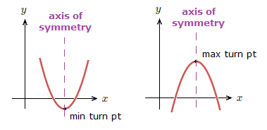
The quadratic equations introduction page mentioned how a quadratic graph can have a maximum or minimum turning point, which dictates the overall shape of the curve.
The curves are also symmetrical, and have an axis of symmetry at the max or min vertex.
We’ll see this with the graphing quadratic functions examples on this page.
But establishing the maximum or minimum turning point is only a part of the process of graphing a quadratic function.
When learning how to approach graphing quadratic functions examples, there is some more information we look to obtain before sketching the correct curve.
Graphing Quadratic Functions Steps:
When we have a quadratic function in standard form.
y = ax^{\tt{2}} + bx + c or f(x) = ax^{\tt{2}} + bx + c
1) Note the nature of a, a > 0 or a < 0 dictates the curve shape.
2) Find the coordinates of the max or min turning point of the curve, (x,y).
We can do this by first finding the x value, which is given by: x = {\text{-}}{\Large{{\frac{b}{2a}}}}
Inputting this value into the function will then give is the y value.
3) Input x = 0 into function to obtain intercept on y-axis.
4) Input y = 0 into function to obtain intercepts on x-axis, if there are any.
Graphing Quadratic Functions Examples
(1.1)
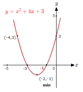
Sketch the graph of the quadratic function y = x^{\tt{2}} + 4x + 3.
Solution
– a > 0, so the curve will have a minimum turning point.
– x = {\text{-}}{\Large{{\frac{b}{2a}}}} => x = {\text{-}}{\Large{{\frac{4}{2(1)}}}} \space = \space {\text{-}}2
y({\text{-}}2) = ({\text{-}}2)^{\tt{2}} + 4({\text{-}}2) + 3 \space = \space 4 \space {\text{--}} \space 8 + 3 \space = \space {\text{-}}1
Minimum turning point coordinates are ({\text{-}}2 , {\text{-}}1).
– Inputting x = 0 into y for the y-intercept.
y(0) = (0)^{\tt{2}} + 4(0) + 3 \space = \space 0 \space {\text{--}} \space 0 + 3 \space = \space 3
y-intercept at (0 , 3).
– Setting y = 0 and solving for the x-intercepts.
x^{\tt{2}} + 4x + 3 = 0
(x + 1)(x + 3) = 0 => x = {\text{-}}1 \space , \space x = {\text{-}}3
Using this information, we can start off by plotting the points we know, and drawing an axis if symmetry.
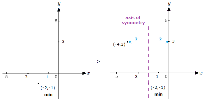
Knowing there is an axis of symmetry at the minimum point, helps us to plot another point on the curve on the opposite side to the y-axis.
Here we move the same distance to the left as the y-intercept to the right, which is 2 units.
(1.2)
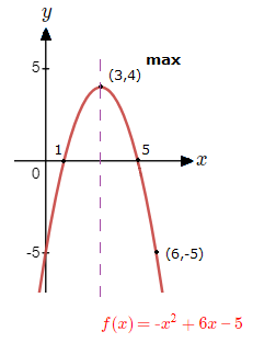
Sketch the graph of the quadratic function f(x) = {\text{-}}x^{\tt{2}} + 6x \space {\text{--}} \space 5.
Solution
– a < 0, so the curve will have a maximum turning point.
– x = {\text{-}}{\Large{{\frac{b}{2a}}}} => x = {\text{-}}{\Large{{\frac{6}{2({\text{-}}1)}}}} \space = \space 3
f(3) = {\text{-}}(3)^{\tt{2}} + 6(3) \space {\text{-}} \space 5 \space = \space {\text{-}}9 + 18 \space {\text{--}} \space 5 \space = \space 4
Maximum turning point coordinates are (3 , 4).
– Inputting x = 0 into f(x) for the y-intercept.
f(0) = {\text{-}}(0)^{\tt{2}} + 6(0) \space {\text{--}} \space 5 \space = \space 0 + 0 \space {\text{--}} \space 5 \space = \space {\text{-}}5
y-intercept at (0 , {\text{-}}5).
– Setting y = 0 and solving for the x-intercepts.
{\text{-}}x^{\tt{2}} + 6x \space {\text{--}} \space 5 = 0
(x \space {\text{--}} \space 1)({\text{-}}x + 5) = 0 => x = 1 \space , \space x = 5
There is now enough information to proceed with sketching the curve of this graphing quadratic functions example.
(1.3)
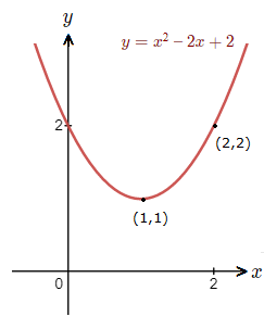
Sketch the graph of the quadratic function y = x^{\tt{2}} \space {\text{--}} \space 2x + 2.
Solution
– a > 0, so the curve will have a minimum turning point.
– x = {\text{-}}{\Large{{\frac{b}{2a}}}} => x = {\text{-}}{\Large{{\frac{{\text{-}}2}{2(1)}}}} \space = \space 1
y(1) = (1)^{\tt{2}} \space {\text{-}} \space 2(1) + 2 \space = \space 1 \space {\text{--}} \space 2 + 2 \space = \space 1
Minimum turning point coordinates are (1 , 1).
– Inputting x = 0 into y for the y-intercept.
y(0) = (0)^{\tt{2}} \space {\text{--}} \space 2(0) + 2 \space = \space 1 \space {\text{--}} \space 0 \space + 2 \space = \space 2
y-intercept at (0 , 2).
Now usually we would set y = 0 and solve to find the x-intercepts.
But we can see that the minimum turning point is (1,1), above the x axis.
So there will be no x-intercepts with the graph of y = x^{\tt{2}} \space {\text{--}} \space 2x + 2 .
This can sometimes be the case with graphing quadratic functions examples.