On this Page:
1. Turning Points
2. Leading Terms, Coefficients
3. Leading Coefficient Test
4. Multiplicity of a Zero
5. Graphing Steps & Example
1. Turning Points
2. Leading Terms, Coefficients
3. Leading Coefficient Test
4. Multiplicity of a Zero
5. Graphing Steps & Example
Here we look at how to approach graphing polynomial functions examples, where we want to try to make as accurate a sketch as we can of a polynomial graph on an appropriate axis.
Some examples of graphing quadratic graphs which are polynomials of degree 2 can be seen here.
When a polynomial is of larger degree though, sometimes we need to do a bit more work for some more information on what the shape of the graph should be.
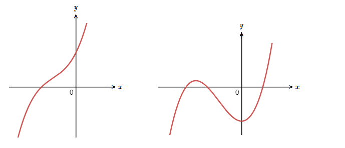
Here are two examples of what a polynomial graph can look like.
Polynomial graphs are smooth graphs and have no holes or breaks in them.
Turning Points
The curves on polynomial graphs are called the ‘turning points’.A polynomial of degree n,
has at most n − 1 turning points on its graph.
So the graph of a polynomial such as f(x) = x^3 + 5x^2 \space {\text{–}} \space 2x + 1,
will have at most 2 turning points.
Leading Terms and Leading Coefficients:
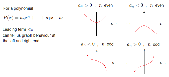
With learning how to deal with graphing polynomial functions examples it’s important to be clear about the leading term and leading coefficient is in a polynomial.For a polynomial, P(x) = a_{n}x^n + a_{n \space {\text{–}} \space 1}x^{n \space {\text{–}} \space 1} + … + a_{1}x + a_0.
a_n is the leading coefficient,
a_{n}x^n is the leading term.
So with g(x) = 2x^3 + x^2 \space {\text{–}} \space 2x + 5,
the leading coefficient is 2, the leading term is 2x^3.
Leading Coefficient Test:
Something called the ‘leading coefficient test’ can help us establish the behaviour of the polynomial graph at each end.As stated, for a polynomial P(x) = a_{n}x^n + a_{n \space {\text{–}} \space 1}x^{n \space {\text{–}} \space 1} + … + a_{1}x + a_0,
the leading term is a_{n}.
There are 4 cases we can have with the leading term, and what it can tell us.
1) a_{n} > 0 \space\space , \space\space n even. The graph will increase with no bound to the left and the right.
2) a_{n} > 0 \space\space , \space\space n odd. The graph will decrease to the left, and increase on the right with no bound.
3) a_{n} < 0 \space\space , \space\space n even. The graph will decrease with no bound to the left and the right.
4) a_{n} < 0 \space\space , \space\space n odd. The graph will increase on the left, and decrease to the right with no bound.
Multiplicity of a Zero:
The multiplicity of a zero is the number of times it appears in the factored polynomial form.For (x \space {\text{–}} \space 5)^3(x + 1)^2 = 0.
The zeros are 5 and {\text{-}}1.
Of which, 5 has multiplicity 3, and {\text{-}}1 has multiplicity 2.
So:
When (x \space {\text{–}} \space t)^m is a factor, t is a zero.
If m is even, the x-intercept at x = t will only touch the x-axis, but not cross it.
If m is odd, the x-intercept at x = t will cross the x-axis.
Also if m is greater than 1, the curve of the polynomial graph will flatten out at the zero.
Graphing Polynomial Functions Examples
Steps
So in light of what we’ve seen so far on this page, to make a sketch of the graph of a polynomial function there are some steps to take.
A) Find the zeros of the polynomial and their multiplicity.
B) Use the leading coefficient test to establish the graph end behaviour.
C) Find the y-intercept, (0,P(0)).
D) Establish the maximum number of turning points there can be, n \space {\text{–}} \space 1.
E) Plot some extra points for some more information of graph shape between the zeros.
Part E) will become more clear in an example.
Example
(1.1)
Sketch the graph of the polynomial f(x) = x^4 \space {\text{–}} \space 3x^3 \space {\text{–}} \space 9x^2 + 23x \space {\text{–}} \space 12.
Solution
Often we are required to find the factors and zeros, but as to concentrate on sketching a graph the polynomial here, we will state them.
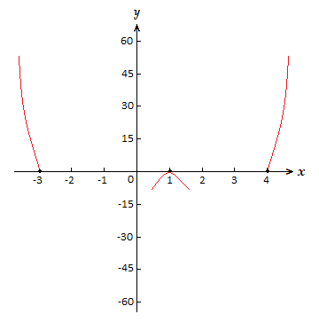
f(x) = x^4 \space {\text{–}} \space 3x^3 \space {\text{–}} \space 9x^2 + 23x \space {\text{–}} \space 12 \space = \space (x \space {\text{–}} \space 1)^{\tt{2}}(x \space {\text{–}} \space 4)(x + 3)
(x \space {\text{–}} \space 1)^{\tt{2}}(x \space {\text{–}} \space 4)(x + 3) \space = \space 0 => x = 1 \space , \space x = 4 \space , \space x = {\text{-}}3
Of the zeros, 1 has multiplicity 2, while 4 and {\text{-}}3 have multiplicity 1.
So the graph will cross the x-axis at –3 and 4, but only touch at 1.
The leading coefficient is 1, which is > 0, and n = 4.
So the graph will increase with no bound past both the left and right ends.
For the y-intercept. f(0) = {\text{-}}12 => (0,-12)
As n = 4, there can be at most 3 turning points, if our graph has any more we have done something wrong somewhere.
With what we know thus far, we can make a start at a sketch of the polynomial graph, on a suitable axis.
Now we look to establish some extra information about graph behaviour between the zeros or other point son the x-axis.
Between 1 and 4. f(3) = {\text{-}}24 \space , \space f(2) = {\text{-}}10
So there is a turning point between 1 and 4.
With n \space {\text{–}} \space 1 = 3, there can only be one more turning point.
Between -3 and 0. f({\text{-}}2) = {\text{-}}54 \space , \space f({\text{-}}\frac{3}{2}) = {\text{-}}51.56
There is a turning point between -3 and 0.
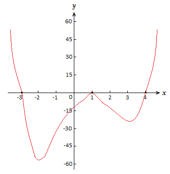
In calculus we can work out more exact turning points and make more exact drawings of polynomial graphs when dealing with graphing polynomial functions examples.
But for a rough sketch of the graph, what we have above gives us a good idea and is fairly accurate.